How to create a Heatmap (II): heatmap or geom_tile
Heatmaps visualise data through variations in colouring.
There are different functions to create a heatmap, one of them is using the heatmap function, but it is also possible to create a heatmap using geom_tile from ggplot2.
The election for one of these function relies on the dataset. Below there is an example developed step by step, to make it clear when it is appropriate to use one function or the other.
Idea
Develop two heat maps using the heatmap function and the geom_tile function, using the same data set. For those interested in following the process step by step, all the information is in my github account:
- Data with the format required for heatmap function.
- Data with the format required for geom_tile function
- R code
- R code for geom_tile
Heatmap using the heatmap function
Our data set is composed of detailed information for three countries – Argentina, Uruguay and Brazil – with 5 different variables -titles, match, points, points_1 (points per game) and performance.
| Team | Titles | Match | Points | Points | Performance |
|---|---|---|---|---|---|
| Argentina | 14 | 41 | 398 | 2,11 | 70,19% |
| Uruguay | 15 | 43 | 358 | 1,82 | 60,58% |
| Brasil | 8 | 35 | 332 | 1,87 | 62,17% |
How to create the heatmap
The dataset on which the heatmap function is going to be applied must be numeric, it usually requires trimming the names of the rows and also making the necessary transformations on each of the variables towards the numerical / integer type.
url <- 'https://raw.githubusercontent.com/frm1789/soccer_ea/master/Example_Data_Matrix_heatmap.csv'
df_matrix <- read_csv(url(url_soccer))

# Order data for titles
df_matrix <- df_matrix[order(df_matrix$Titles, decreasing = FALSE),]
df_matrix <- data.frame(df_matrix)

#removing names of the teams.
row.names(df_matrix) <- df_matrix$Team
df_matrix <- df_matrix[,-1]

options(digits=2)
df_matrix$Points_1 <- sub(',', '.', df_matrix$Points_1)
df_matrix$Points_1 <- as.double(df_matrix$Points_1)

# transformation to numeric for column "Performance"
df_matrix$Performance = substr(df_matrix$Performance,1,nchar(df_matrix$Performance)-1)
df_matrix$Performance <- sub(',', '.', df_matrix$Performance)
df_matrix$Performance <- as.double(df_matrix$Performance)
df_matrix$Performance <- log(df_matrix$Performance)

small_matrix <- data.matrix(df_matrix)

# Creation of heatmap
america_heatmap <- heatmap(small_matrix, Rowv=NA,
                           Colv=NA, col = brewer.pal(9, "Blues"), scale="column",
                           margins=c(2,6))
Results
Let’s analyze the image:
- In the Title column, we have Uruguay (15), Argentina (14) and Brazil (8): the difference in color that we appreciate between Uruguay and Argentina is minimal, but if we compare it with Brazil we see the 7-8 points of difference.
- In the Match column, we have Uruguay (43), Argentina (41) and Brazil (35): again between Uruguay and Argentina there is a minimum difference of colors, much more noticeable with Brazil.
Following the same line of reasoning we can see the same thing for the other variables, that is, we compare each variable in relation to the values that it takes for Uruguay, Argentina and Brazil, and understanding that the higher values are darker, and the but lower values are clearer.

Heatmap using geom_tile function (ggplot2) – Part 1
We will generate the heatmap using the geom_tile function from ggplot2.
Data with the required format for geom_tile
| country | metric | value |
|---|---|---|
| Uruguay | Titles | 15 |
| Uruguay | Match | 43 |
| Uruguay | Points | 358 |
| Uruguay | Points_1 | 1.82 |
| Uruguay | Performance | 4.1 |
| Argentina | Titles | 14 |
| Argentina | Match | 41 |
| Argentina | Points | 398 |
| Argentina | Points_1 | 2.11 |
| Argentina | Performance | 4.3 |
| Brasil | Titles | 8 |
| Brasil | Match | 35 |
| Brasil | Points | 332 |
| Brasil | Points_1 | 1.87 |
| Brasil | Performance | 4.1 |
How to create the heatmap with geom_tile
The horizontal view was added to make the comparison between both resulting images easier, and the minimal theme was added to improve the aesthetics.
library(ggplot2)

url_soccer <- 'https://raw.githubusercontent.com/frm1789/soccer_ea/master/Example_Data_format_ggplot_geom_tile.csv'
df_exa <- read_csv(url(url_soccer))
ggplot(data = df_exa, aes(x = df_exa$country, y = df_exa$metric)) +
  geom_tile(aes(fill = df_exa$value)) +
  coord_flip() +
  scale_fill_gradient(low = "#C6DBEF", high = "#08306B") +
  theme_minimal()
Results
We have a totally different image, different from the obtained using the heatmap funcion.

The results using geom_tile and heatmap are different. Why?
Because each of the variables in this dataset have different units with very different ranges and that do not have any type of relationship: matches, titles, points, performance, all have different units of measurement, there is no common point of comparison between them.
To use geom_tile, we need all variables in the dataset expressed in the same unit.
How heatmap function works?
A heat map (or heatmap) is a graphical representation of data where the individual values contained in a matrix are represented as colors. In our case, since the very different nature of each variable, we are using scale = "column", indicating that the values should be centered and scaled in the column direction. The default value for this parameter is "none"
How geom_tile function works?
In its description we can read: tile plane with rectangles. To tile a rectangle is to divide it up into smaller rectangles or squares. Each of the smaller rectangles or squares is called a tile. The function assumes all the dataset expressed in the same unit.
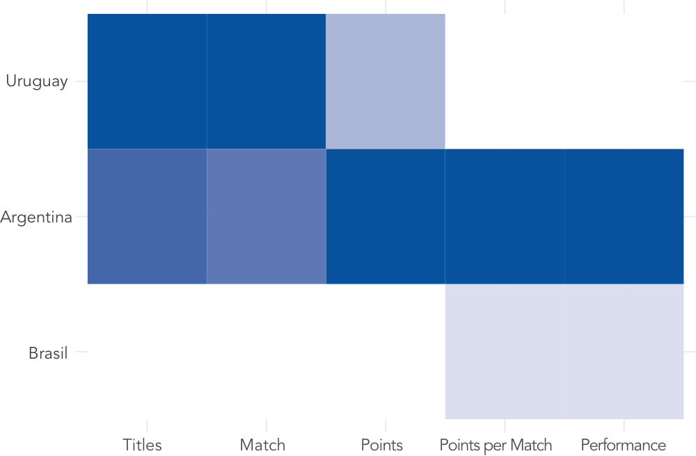
Heatmap using the geom_tile function (ggplot2) – Part 2
We will generate the heatmap using the geom_tile function from ggplot2, but in this case we will be sure that we are applying the geom_tile for each column. The function rescale will be used to express all the values in the scale.
Code
url_soccer <- 'https://raw.githubusercontent.com/frm1789/soccer_ea/master/AmericaCupData_small.csv'
df_soccer <- read_csv(url_soccer)

# Everything to numeric
options(digits=2)
df_soccer$Points_1 <- sub(',', '.', df_soccer$Points_1)
df_soccer$Points_1 <- as.double(df_soccer$Points_1)
df_soccer$Performance = substr(df_soccer$Performance,1,nchar(df_soccer$Performance)-1)
df_soccer$Performance <- sub(',', '.', df_soccer$Performance)
df_soccer$Performance <- as.double(df_soccer$Performance)
df_soccer$Performance <- log(df_soccer$Performance)


# Reshape for geom_tile format
df_soccer <- reshape2:::melt.data.frame(df_soccer)

# Use of rescale
tableau.m <- ddply(df_soccer, .(variable), transform, rescale = rescale(value))

# Maintain the order
tableau.m$Team <- factor(tableau.m$Team, c("Brasil", "Argentina", "Uruguay"))
tableau.m$variable <- factor(tableau.m$variable, c("Titles", "Match", "Points", "Points_1", "Performance"))

# Plot the visualization
ggplot(tableau.m, aes(variable, Team, fill = rescale)) +
  geom_tile(show.legend = FALSE) +
  scale_fill_gradient(low = "white", high = "steelblue") +
  theme_minimal()
Results
Conclusions
The heatmap function provides very straight way to create a heatmap. It is practical, clean and simple. It could be said that it is the most appropriate way to create a heat map.
Nevertheless, through the use of geom_tile, you are using ggplot2, and all the facilities about aesthetics. The downside is the extra work with the format of the dataset and the use of factor to maintain the order.
Bibliography
This work would have been impossible, without the information from the next sources. If there is an error in the interpretation is exclusively mine.
- TilingRectangles
- How to create a heatmap per column
- How create a heatmap
- You probably don’t understand a heatmap